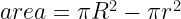
A Variation on Bertrand’s Paradox (with Python simulation code)

A friend recently challenged me with this problem she found at a math competition:

It is actually quite a simple problem, that only requires some knowledge of the Pythagorean theorem, the challenge is recognizing that you have enough information to solve the problem even though you cannot compute the radius of either circle.

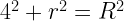
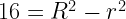
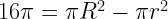
Just put in a right triangle, and call the radius of the smaller circle r and the radius of the larger circle R.

$area = \pi R^2 - \pi r^2$
$4^2 + r^2 = R^2$
$16 = R^2 - r^2$
$16\pi = \pi R^2 - \pi r^2$
$area = 16\pi$

Anyways, I was thinking about this problem as well as the Buffon’s needle problem, when I thought of this (seemingly simple) combination.

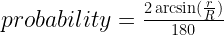
Suppose you have two concentric circles of known radii and you randomly choose a chord of the larger circle. What is the probability of the chord passing through the smaller circle?

The orange chords are those that intersect the center circle and the blue are those that do not.

I figured that this essentially the same as the Buffon’s needle problem (where you determine the probability that a needle crosses a set of parallel lines on the floor) and could be solved similarly using angles.

Since the circle has infinite rotational symmetry, we can choose one endpoint for our chord without loss of generality (as a point on the circle can be transformed into any other point via a rotation). Then, by randomly selecting the other endpoint, we can define a chord between the two points. If this chord is within $\theta$ of horizontal, it will pass through the smaller circle. The total range of angles possible is 180 degrees and only chords passing through 2 $\theta$ of this range pass through the center circle so $probability = \frac{2\theta}{180}$ .

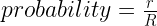
To get theta in terms of R and r (which is what we want our probability in terms of) we set up a right triangle:

$\sin(\theta) = \frac{r}{R}$
$2\theta = 2\arcsin(\frac{r}{R})$

So $probability = \frac{2\arcsin(\frac{r}{R})}{180}$

Let’s call this Method 1: Endpoint Method, because it relies on the selection of two random endpoints to define a random chord.

I thought this was quite elegant and showed it to my friend the next day at school. She, however, quickly thought of a simpler solution which seemed equally valid.

Instead of fixing one endpoint of the chord, she suggested giving it a fixed angle. Looking at one angle is representative just like choosing a particular endpoint, again because of rotational symmetry. So, for instance, we can look only at chords parallel to the y-axis.

This makes it clear that $probability = \frac{r}{R}$
We’ll call this Method 2: Radius Method because we choose a random radius for our chords to be perpendicular to.

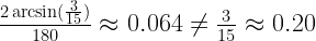
At first, I thought these two solutions must be equal and that 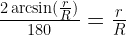$\frac{2\arcsin(\frac{r}{R})}{180} = \frac{r}{R}$ must be a mathematical identity. But if you plug in some numbers, say R = 15 and r = 3, you realize that these are most definitely not equal.

$\frac{2\arcsin(\frac{3}{15})}{180} \approx 0.064 \neq \frac{3}{15} \approx 0.20$

While trying to reconcile this, I came up with yet another method to solve the problem which yielded yet another answer!

This method utilizes the fact that a chord passes through the inner circle if and only if the chord’s midpoint is in the inner circle.

Also, except for chords with a midpoint in the exact center of the circle (randomly choosing the center has a probability of zero and can be ignored) any chord can be defined by its midpoint by drawing the radius passing through the midpoint and the chord as perpendicular.

So we can generate random chords by selecting random midpoints and a chord will pass through the center circle if its midpoint is in the circle. Therefore, the probability of a chord passing through the center circle should be the ratios of the areas of the circles or $latex probability = \frac{r^2}{R^2} &s=2$.

We’ll call this Method 3: Midpoint Method, for fairly obvious reasons.

Someone pointed out to me that each of the three methods relied on a different way of randomly generating a chord:

Method 1: Specify two random points on the large circle’s perimeter. This can be done by randomly choosing two angles $\theta_1$ and $\theta_2$ between 0 and 360 degrees.

Method 2: Specify a random point on the large circle’s perimeter (to determine a radius) and a random length along that radius. This can be done by randomly choosing an angle $\theta_1$ from 0 to 360 degrees and a length L from 0 to R.

Method 3: Specify a random point within the large circle. This can be done by choosing a random x and y coordinate from -R to R and selecting again if (x,y) falls outside the circle.

Each method requires two randomly generated values to determine a chord, but what those values represent varies.

Still, its unclear why these differences should affect the probability. Each one of the three methods can generate every possible chord within the larger circle. And since there are infinite possible chords, the probability of generating any one specific chord is zero for all three methods (here’s an explanation). It seemed intuitive that this should mean that all three methods were equivalent.

When I searched this problem I found that it was essentially the equivalent of Bertrand’s paradox (named for its creator: Joseph Bertrand), which uses a circle and an inscribed equilateral triangle rather than concentric circles.

The resolution to Bertrand’s paradox is that our intuitions about the three methods being equal is incorrect. They actually generate three different probability distributions of chords in the circle. This is hard to imagine unless you can see it, so I wrote some code in Python to illustrate the disparate results of the three methods. (code included at end of post, in case you want to mess around with it)

Each of these images shows 100 random chords on a large circle with radius 15 units and calculates the theoretical (according to the disparate formulas) and actual (according to the simulation) probabilities that the chord passes through a smaller concentric circle of radius 3.

These images show that even though all three methods can each generate every possible chord in the circle, they aren’t all the same. This is perhaps clearest from the chord distribution generated by the midpoint method, where there are few chords passing close to the center of the circle and many more closer to the edges of the large circle. The “paradox” is a result of unevenness between the distributions of the three methods.

So which of the three is the “correct” method?
In one sense, all three are correct. It merely depends on how the original problem defines “a randomly chosen chord”. The answer depends on whether the chord is selected by its endpoints, an angle, or its midpoint. The problem need to be more specific in order to be “well-posed” and possess a unique solution.

This is a fairly unsatisfying answer however, and it is possible to dive deeper. When we think of “random” we usually think uniformly distributed, meaning every outcome should occur with the same frequency. For example, a coin that lands on heads two out of three times has a skewed probability distribution while a fair coin has a uniform one. Either of these coins does land on heads some of the time and tails some of the time, but we prefer the fair coin.

So then we can ask, which of the three methods represents the “fair coin”?
This question actually has an answer: it has been proven to be Method 2: Radius Method. This is the method that represents throwing a stick onto a circle inscribed on the floor and it is the only possible method that generates a uniform distribution of chords on a circle. This means that no matter where you are in the circle (one can imagine sampling random unit squares) the same (on average) number of chords will pass through that area. The Radius Method was proven to be the only method that generates such a uniform distribution by Edwin Jaynes in his 1973 paper “The Well-Posed Problem”. Jayne’s proof gets quite involved but you can perhaps convince yourself that Method 2 is the correct method by seeing how it appears to produce a homogeneous shading of chords in the circle while methods 1 and 3 do not.

Python Simulation Code:
If you are a novice to programming/Python, all you need to run this code is to download Anaconda with Python and all the packages you need will already be installed (matplotlib and scipy specifically).

Code Link