Computer Science – iRashida

Optimal Routes for your Data

An overview of currently used routing protocols and a investigation of a mathematically optimal alternative. Visualizations and code included! Post in collaboration with Akshay Yeluri.

When you send an email, do you ever wonder how that data makes its way from your phone or computer to whoever you are sending it to? This question gets to the core of how the internet works, which in all its power and magic, is essentially a data transfer system. But it is a ridiculously huge data transfer system – it’s estimated that global internet traffic is around 122,000 petabytes per month (for reference, a petabyte is about 10,000 4k movies worth of data). This term, I took a class called Communication Networks that focused on understanding the protocols that make the internet work under the hood. I found a good layperson’s overview of some of these topics in this Medium article, in case you’re also interested. Personally, I was particularly fascinated by routing protocols, which determine the paths through the network that packets (bits of data) take to make it to their appropriate destinations.

What are Routing Protocols?

First, a bit of background is needed to understand routing protocols. There exists some collection of hosts (people’s personal devices) which are the sources and destinations for the data packets. A limited number of hosts can connect to a single router – which is a device whose job it is to get packets to their correct destination. Each router is also connected to a limited number of other routers. All together, these connections form a network of millions of routers that connect billions of hosts.

This image shows a small network of routers connected to hosts. In future visualizations, we will only show the routers in the graph for simplicity. Since each host connects to only one router, finding a path from Host 1 to Host 3 (for example) is equivalent to finding a path from router A to router C.

Now, the problem that routing protocols try to solve can be formulated as follows: When host A sends a packet to host B, what path should that packet take to get to B as fast as possible? Once these paths are decided for every pair of hosts, the routers ensure that packets (which are tagged with their destination) actually travel along these routes. Each router has a routing table which tells it which one of its neighbors to route each packet to (based on the packet’s destination). Routing tables fully determine the path that every packet in the network will take, so we can reformulate our problem as: What should the routing tables be so that packets get to their destinations as fast as possible?

It remains to ask: What makes a certain path fast or slow? Initially you might think that it’s solely based on the number of links on the path (more links = slower) and to some extent this is true. However, it is also true that increased traffic along a connection makes it slower due to queuing delay. You can think of queueing delay as the time the packets have to stand in line before being sent along a busy link. This adds complexity to the problem, as the choice of routing tables affects how many packets are sent along a particular link, and therefore affects the average travel time of the packets (a.k.a. the average packet delay). This means that a good routing protocol will make trade-offs between choosing the shortest paths and avoiding routing packets along highly trafficked links.

Dynamic Shortest Paths Routing

The routing protocol that is actually used in the internet is a variation of dynamic shortest paths routing. Shortest paths is a bit of a misnomer, as it is not actually shortest paths routing but fastest paths routing. At every timestep, the protocol involves constructing the graph consisting of all the routers in the network and their connections, and assigning each directed edge a weight. This weight is the packet delay along the link calculated using the current routing table and the data traffic from the previous timestep. Note that both of these are required to calculate the total traffic along the link, and therefore the packet delay.

Once this graph is constructed, an algorithm like Floyd-Warshall is used to calculate all-pairs shortest paths for the weighted graph. This corresponds to all-pairs fastest paths for the network, since the weight on each edge is the time to travel along that edge. So minimizing the weighted length of the path from A to B minimizes the travel time of a packet going from A to B. The routing tables in the network are then updated to match the shortest paths found by Floyd-Warshall.

Shortest path from A to F on the weighted graph is shown in blue. Note that there is a ‘shorter’ path (A, B, D, F) but that has higher total edge weight.

The ‘dynamic’ in the name of this protocol comes from the fact that it updates the routing tables at every timestep based on the traffic of the previous timestep. This means that it can naturally accommodate traffic distributions that change over time. We would hope that under stationary traffic distributions, dynamic shortest paths routing would eventually converge, however this is not the case. In fact, a major disadvantage of dynamic shortest paths routing is that the routing tables can oscillate wildly between timesteps. This behavior comes from the fact that the algorithm generally chooses to use links that were lightly trafficked (and therefore fast) in the previous timestep, but does not consider that this choice will cause those very links to now be heavily trafficked (and therefore slow). The variants on dynamic shortest paths routing that are used in practice exist mainly to address this problem. If you would like to know more about these variants, an interesting paper on preventing oscillations in routing tables can be found here.

Visualizations (Shortest Paths)

Code on Github

The left image shows how the average packet delay changes with steps of the dynamic shortest paths protocol. We see the oscillatory behavior characteristic of this protocol. The right image shows how the total traffic on each link evolves, for example we can see the (1, 2) link becoming more heavily trafficked and the (1, 0) link being used less as the simulation progresses. The total traffic graph is essentially what Floyd-Warshall is run on in each step of the protocol, as heavily trafficked links have higher weight and are slower.

This shows the evolution of the routing tables with respect to each destination node in the network (average packet delay is also shown on the bottom right). We can see that for destination 0, node 3 oscillates between sending data to node 2 and node 1. This makes sense given that when node 3 routes to node 2 the link (3, 2) becomes heavily trafficked (traffic of 4) and when node 3 routes to node 1 the link (3, 1) becomes heavily trafficked (traffic of 6). This from the traffic video above.

Probabilistic Routing

An interesting alternative to the routing protocols used in practice can be found in the paper “A Minimum Delay Routing Algorithm Using Distributed Computation” by Robert Gallagher (1977). We can consider the routing tables we have talked about so far to be deterministic: once the routing table is fixed, all packets traveling from A to B follow the same path. Gallagher proposes routing tables that we will call ‘probabilistic’, meaning that all traffic traveling from A to B does not necessarily take the same route (even within a timestep). Given a packet at router A destined for B, the packet’s next location is drawn from a probability distribution over neighbors of A. This probability distribution is defined in the routing table for A.

The benefit of this formulation of routing tables is that it allows more flexibility in dividing traffic evenly across the network, and therefore allows for less packet delay. In fact, Gallagher gives a protocol for updating probabilistic routing tables that he proves always converges to the minimal average packet delay given stationary traffic distributions. This means that it’s relatively easy to make probabilistic routing optimal! However, the trade-off is that probabilistic routing tables are more complicated, since implementing them requires every router to be able to sample from a probability distribution.

As our project for Communication Networks, we implemented Gallagher’s protocol and checked that it converged to the optimal routing tables by also performing numerical minimization of the average packet delay (using scipy). Our code for this project can be found at our GitHub. Interestingly, we found a small network (only 4 nodes!) where the best probabilistic routing table significantly outperforms the best deterministic routing table. This means that using probabilistic routing tables could prove worthwhile in networks where minimizing packet delay is very important and simple network design is less of a consideration.

Visualizations (Gallagher)

Code on Github

The left image shows how the average packet delay changes with steps of the Gallagher protocol. We can observe convergence to the minimum average packet delay solution. We also notice that the total traffic on each link (shown on the right) is not always an integer value. This is because the non-integer values in the routing tables allow the expected number of sent packets along a link to be a non-integer.

This shows the evolution of the routing tables with respect to each destination node in the network (average packet delay is also shown on the bottom right). Going back to the example from the shortest paths case, we can see that node 3 routes some fraction of traffic destined for node 0 to node 1 and some fraction to node 2. This is why this protocol is able to converge instead of oscillating like the previous example.

A Variation on Bertrand’s Paradox (with Python simulation code)

Understanding the importance of a well-posed problem by examining a math problem with 3 different “correct” solutions.

A friend recently challenged me with this problem she found at a math competition:

It is actually quite a simple problem, that only requires some knowledge of the Pythagorean theorem, the challenge is recognizing that you have enough information to solve the problem even though you cannot compute the radius of either circle.

Just put in a right triangle, and call the radius of the smaller circle r and the radius of the larger circle R.

$area = \pi R^2 - \pi r^2$
$4^2 + r^2 = R^2$
$16 = R^2 - r^2$
$16\pi = \pi R^2 - \pi r^2$
$area = 16\pi$

Anyways, I was thinking about this problem as well as the Buffon’s needle problem, when I thought of this (seemingly simple) combination.

Suppose you have two concentric circles of known radii and you randomly choose a chord of the larger circle. What is the probability of the chord passing through the smaller circle?

The orange chords are those that intersect the center circle and the blue are those that do not.

I figured that this essentially the same as the Buffon’s needle problem (where you determine the probability that a needle crosses a set of parallel lines on the floor) and could be solved similarly using angles.

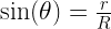
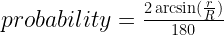
Since the circle has infinite rotational symmetry, we can choose one endpoint for our chord without loss of generality (as a point on the circle can be transformed into any other point via a rotation). Then, by randomly selecting the other endpoint, we can define a chord between the two points. If this chord is within $\theta$ of horizontal, it will pass through the smaller circle. 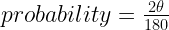The total range of angles possible is 180 degrees and only chords passing through 2 $\theta$ of this range pass through the center circle so $probability = \frac{2\theta}{180}$ .

To get theta in terms of R and r (which is what we want our probability in terms of) we set up a right triangle:

$\sin(\theta) = \frac{r}{R}$
$2\theta = 2\arcsin(\frac{r}{R})$

So $probability = \frac{2\arcsin(\frac{r}{R})}{180}$

Let’s call this Method 1: Endpoint Method, because it relies on the selection of two random endpoints to define a random chord.

I thought this was quite elegant and showed it to my friend the next day at school. She, however, quickly thought of a simpler solution which seemed equally valid.

Instead of fixing one endpoint of the chord, she suggested giving it a fixed angle. Looking at one angle is representative just like choosing a particular endpoint, again because of rotational symmetry. So, for instance, we can look only at chords parallel to the y-axis.

This makes it clear that $probability = \frac{r}{R}$
We’ll call this Method 2: Radius Method because we choose a random radius for our chords to be perpendicular to.

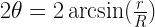
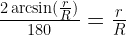
At first, I thought these two solutions must be equal and that $\frac{2\arcsin(\frac{r}{R})}{180} = \frac{r}{R}$ must be a mathematical identity. But if you plug in some numbers, say R = 15 and r = 3, you realize that these are most definitely not equal.

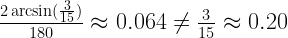
$\frac{2\arcsin(\frac{3}{15})}{180} \approx 0.064 \neq \frac{3}{15} \approx 0.20$

While trying to reconcile this, I came up with yet another method to solve the problem which yielded yet another answer!

This method utilizes the fact that a chord passes through the inner circle if and only if the chord’s midpoint is in the inner circle.

Also, except for chords with a midpoint in the exact center of the circle (randomly choosing the center has a probability of zero and can be ignored) any chord can be defined by its midpoint by drawing the radius passing through the midpoint and the chord as perpendicular.

So we can generate random chords by selecting random midpoints and a chord will pass through the center circle if its midpoint is in the circle. Therefore, the probability of a chord passing through the center circle should be the ratios of the areas of the circles or $latex probability = \frac{r^2}{R^2} &s=2$.

We’ll call this Method 3: Midpoint Method, for fairly obvious reasons.

Someone pointed out to me that each of the three methods relied on a different way of randomly generating a chord:

Method 1: Specify two random points on the large circle’s perimeter. This can be done by randomly choosing two angles $\theta_1$ and $\theta_2$ between 0 and 360 degrees.

Method 2: Specify a random point on the large circle’s perimeter (to determine a radius) and a random length along that radius. This can be done by randomly choosing an angle $\theta_1$ from 0 to 360 degrees and a length L from 0 to R.

Method 3: Specify a random point within the large circle. This can be done by choosing a random x and y coordinate from -R to R and selecting again if (x,y) falls outside the circle.

Each method requires two randomly generated values to determine a chord, but what those values represent varies.

Still, its unclear why these differences should affect the probability. Each one of the three methods can generate every possible chord within the larger circle. And since there are infinite possible chords, the probability of generating any one specific chord is zero for all three methods (here’s an explanation). It seemed intuitive that this should mean that all three methods were equivalent.

When I searched this problem I found that it was essentially the equivalent of Bertrand’s paradox (named for its creator: Joseph Bertrand), which uses a circle and an inscribed equilateral triangle rather than concentric circles.

The resolution to Bertrand’s paradox is that our intuitions about the three methods being equal is incorrect. They actually generate three different probability distributions of chords in the circle. This is hard to imagine unless you can see it, so I wrote some code in Python to illustrate the disparate results of the three methods. (code included at end of post, in case you want to mess around with it)

Each of these images shows 100 random chords on a large circle with radius 15 units and calculates the theoretical (according to the disparate formulas) and actual (according to the simulation) probabilities that the chord passes through a smaller concentric circle of radius 3.

These images show that even though all three methods can each generate every possible chord in the circle, they aren’t all the same. This is perhaps clearest from the chord distribution generated by the midpoint method, where there are few chords passing close to the center of the circle and many more closer to the edges of the large circle. The “paradox” is a result of unevenness between the distributions of the three methods.

So which of the three is the “correct” method?
In one sense, all three are correct. It merely depends on how the original problem defines “a randomly chosen chord”. The answer depends on whether the chord is selected by its endpoints, an angle, or its midpoint. The problem need to be more specific in order to be “well-posed” and possess a unique solution.

This is a fairly unsatisfying answer however, and it is possible to dive deeper. When we think of “random” we usually think uniformly distributed, meaning every outcome should occur with the same frequency. For example, a coin that lands on heads two out of three times has a skewed probability distribution while a fair coin has a uniform one. Either of these coins does land on heads some of the time and tails some of the time, but we prefer the fair coin.

So then we can ask, which of the three methods represents the “fair coin”?
This question actually has an answer: it has been proven to be Method 2: Radius Method. This is the method that represents throwing a stick onto a circle inscribed on the floor and it is the only possible method that generates a uniform distribution of chords on a circle. This means that no matter where you are in the circle (one can imagine sampling random unit squares) the same (on average) number of chords will pass through that area. The Radius Method was proven to be the only method that generates such a uniform distribution by Edwin Jaynes in his 1973 paper “The Well-Posed Problem”. Jayne’s proof gets quite involved but you can perhaps convince yourself that Method 2 is the correct method by seeing how it appears to produce a homogeneous shading of chords in the circle while methods 1 and 3 do not.

Python Simulation Code:
If you are a novice to programming/Python, all you need to run this code is to download Anaconda with Python and all the packages you need will already be installed (matplotlib and scipy specifically).

Code Link